
Microstrip and stripline are the two transmission-line structures every high-frequency PCB is built from, and most of the decisions that determine their impedance are made before fabrication starts. This article walks the design sequence from structure choice to release for production, and then states what the fabricator must actually control — trace width, dielectric height and copper thickness — because the impedance of a finished line is set by those three numbers, not by the simulation that predicted them.
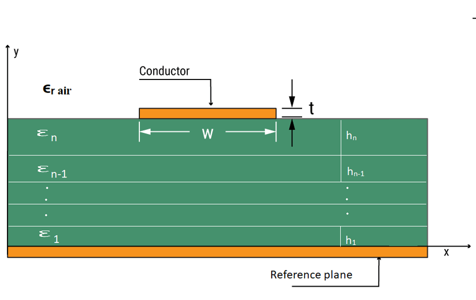
What the Two Structures Actually Are
Both structures need correcting from the usual short definitions, because the errors compound later.
Microstrip is an outer-layer conductor running over a single reference plane. The field lives partly in the laminate and partly in air, so the effective dielectric constant is lower than the laminate Dk — on a Dk 3.66 material, roughly 2.85 for a 50 Ω line. Signals travel faster and structures are cheaper to etch, but the field is exposed: any solder mask, conformal coating or metal object above the trace changes its impedance.
Stripline is not “two parallel conductors”, as it is sometimes described. It is a single conductor buried between two reference planes, fully inside the dielectric. The field is homogeneous, the effective Dk equals the laminate Dk, radiation is zero and isolation from other layers is excellent. The price is geometry: at the same laminate thickness a stripline must be much narrower, which makes it far more sensitive to etch error.
| Property | Microstrip | Stripline |
|---|---|---|
| Location | Outer layer, over one reference plane | Inner layer, between two reference planes |
| Dielectric seen by the field | Mixed — laminate below, air above | Homogeneous laminate |
| Effective Dk (Dk 3.66 material) | ~2.85 | 3.66 |
| 50 Ω width, 0.254 mm dielectric | ~0.56 mm | ~0.23 mm (0.508 mm plane spacing) |
| Etch error ±25 µm → impedance error | about ±2.8% | about ±6.8% |
| Radiation and EMI | Some field in air; edges radiate | None — fully shielded |
| Reference planes required | 1 | 2 |
The structural comparison frames every step that follows: microstrip is cheap, fast and exposed; stripline is quiet, slow and intolerant of manufacturing error.
Step 1 — Fix the Impedance Target and Its Window
Most RF work targets 50 Ω single-ended; 75 Ω survives in video and some antenna feeds, and 100 Ω paired lines handle most differential standards. What matters more than the number is the tolerance window, because the window is what the fabricator quotes against.
A ±10% window on 50 Ω spans 45–55 Ω, and each physical parameter claims a share of it. On a 0.254 mm hydrocarbon laminate, dielectric thickness ±10% alone moves a 50 Ω microstrip by about ±6% — most of the window. Etch error of ±25 µm adds roughly ±2.8% on a 0.56 mm line, and a ±0.05 Dk spread adds under 1%. The contributions add in quadrature to roughly 6.6%, which is why the impedance budget belongs to the stack-up, not to the schematic.
Define the window per line class at this step, in writing. A fabricator who receives “50 Ω” without a window will apply a house default, and the house default may not match what the transceiver at the end of the line assumes.
Step 2 — Choose the Structure and Its Layer Position
The choice is usually made by one dominant requirement:
| If the design needs… | Choose | Why |
|---|---|---|
| Lowest loss per millimetre | Microstrip | Effective Dk below the laminate Dk lowers both dielectric and conductor terms; wide trace keeps copper loss down |
| Isolation from other circuits | Stripline | Fully enclosed field; no radiation, no coupling to components above |
| Direct component launch | Microstrip | Components mount on the same layer; no via transition at the launch |
| Routing density | Stripline | Inner layers, protected; the narrow width packs more lines per layer |
| Long routed runs, e.g. antenna feed networks | Microstrip | No via transitions; every stripline transition adds a discontinuity |
| Mil-aero or high-isolation backplanes | Stripline | Shielding and crosstalk margins outweigh the loss penalty |
Count reference planes before committing: every stripline layer needs a plane on both sides, so n stripline layers require n+1 planes. A four-layer board offers two impedance layers, both microstrip; meaningful stripline capability starts at six layers. This arithmetic is the layer-count rule described in the design-steps guide.
Step 3 — Compute Width from the Right Dk
Width and spacing come from closed-form equations or a field solver, but the input Dk must be the one the fabricator holds to. Laminates publish a process Dk at one frequency and a design Dk across a band, and they differ: RO3010 is 10.2 as processed and 11.20 in design tables. Solving with the wrong one shifts every electrical length by several per cent, as explained in the parameter breakdown.
| Laminate Dk | 50 Ω microstrip W/h | Effective Dk | Guided wavelength at 10 GHz |
|---|---|---|---|
| 2.20 (5880, TLY-5) | 3.11 | 1.87 | 21.9 mm |
| 3.00 | 2.54 | 2.42 | 19.3 mm |
| 3.38 (RO4003C) | 2.33 | 2.67 | 18.3 mm |
| 3.66 (RO4350B) | 2.21 | 2.85 | 17.7 mm |
| 10.2 / 11.20 (RO3010) | 0.85 | 7.41 | 11.0 mm |
Two consequences worth noting. On high-Dk material the 50 Ω trace is barely wider than the dielectric is thick, so the same ±25 µm etch variation is a much larger percentage of the line — high-Dk materials are size decisions, not low-loss decisions. And because microstrip sits in mixed dielectric, anything deposited on the trace shifts it: 25 µm of solder mask over a 0.127 mm PTFE microstrip pulls 50 Ω down by roughly 3 Ω, while the same mask on 0.508 mm moves it under 1 Ω. Model the mask, or specify an opening over the RF trace.
Step 4 — Route Against the Reference, Not Just Short
Short traces matter, but the reference plane matters more. Three routing rules that production cannot repair afterwards:
- Never cross a plane split. A signal crossing a gap in its reference plane has no defined return path; the return detours and the crossing point becomes a radiating, dispersive discontinuity. Route around, or add stitching capacitance at the crossing.
- Keep spacing at three dielectric heights or more between RF lines. Crosstalk is set by the s/h ratio, not by absolute spacing: on thin laminates the field is confined close to the trace, so 3×h is usually enough isolation; on thick dielectrics the same absolute distance couples far more.
- Price the via before using it. A through-via on a 1.6 mm board leaves a stub resonating near 23 GHz — on a 2.0 mm board near 19. Below those frequencies the stub is a small parasitic; above, it is a notch in the passband. Back-drilling or blind vias are the fix, and both cost money the layout should have anticipated.
Layer transitions on stripline runs deserve special attention: each transition microstrip-to-stripline adds a via discontinuity, and a feed network built on inner layers can accumulate several. The loss budget in the next section is what should have priced those vias.
Step 5 — Simulate the Board as It Will Be Built
Solvers such as HFSS or ADS are standard at this step, but the model that predicts the measured board is the one that includes the as-built geometry, not the nominal layout:
- The finish, because it is the conductor. At 10 GHz the skin depth in copper is 0.65 µm, and the 3–6 µm nickel layer of an ENIG finish is where the current actually flows, at twice the surface resistance of copper. On a low-loss laminate such as 5880 or TLY-5, where copper loss already dominates the dielectric term, ENIG can add 30–50% to insertion loss; on FR-4 it changes almost nothing.
- The mask, as above — 1–3 Ω on thin microstrip, and its own loss tangent of 0.02–0.03 is twenty times the laminate’s on a low-Df material.
- Copper roughness. On low-loss laminates the conductor term is 0.04–0.07 dB/in at 10 GHz, so foil type (standard, RTF, VLP) is no longer a procurement detail.
Then record what was modelled. The single most common simulation-versus-measurement gap on high-frequency work is a model of bare copper compared against a finished, masked board — a gap of several ohms that looks like a fabrication error but is a modelling choice.
What Production Must Control While Making These Lines
The design fixes geometry; three process numbers decide whether the finished line meets it:
| Control | What it does to impedance | How it is held |
|---|---|---|
| Etched trace width | Every 1% of width is about 0.62% of impedance; fine lines lose proportionally more to undercut | Etch compensation by copper weight; 0.5 oz for lines under 0.15 mm; LDI registration |
| Dielectric height h | The dominant term — ±10% in thickness is ±6% in impedance | Pressed-height specification, not nominal foil thickness; coupon TDR verification |
| Copper thickness | Sets the conductor term and the undercut budget; 2 oz on a 0.1 mm line shifts 113 Ω designs by +11% | Copper weight chosen at design time; plating thickness recorded per panel |
The fabricator verifies these on a coupon in the same lamination cycle as the product, measured by TDR — the closed loop described in the impedance-control guide. A designer can shortcut surprises by stating the tolerance window, the copper weight and the mask allowance explicitly in the design files.
Temperature: the Phase Budget Most Designs Skip
Material properties move with temperature, and the effect that reaches the system is phase, not attenuation. A 100 mm stripline at 10 GHz carries between roughly 1,800 and 2,300 degrees of accumulated phase; a TCDk of +50 ppm/°C across a −50 to +150 °C range shifts it by about 11 degrees, and a negative-TCDk PTFE by about 22.
For radar, phased arrays and any beam-forming network, 11–22 degrees of drift is a calibration item, not a footnote. The mitigation is material selection at the start — matched TCDk across the materials in one stack — because nothing in fabrication corrects it afterwards. Designers working across temperature should treat TCDk as a first-class stack parameter, as covered in the impedance and layer-stack guide.
Common Issues and What Actually Fixes Them
The standard list of “issues and solutions” is mostly right, but the fixes are frequently stated at the wrong level. The table re-anchors each one:
| Symptom | Common description | What actually fixes it |
|---|---|---|
| Signal reflection | Mismatched impedance | Usually an unmodelled discontinuity: the mask, the finish, a layer transition or a pad on the line — not the nominal trace width |
| Crosstalk | Adjacent-trace interference | Spacing as a ratio to dielectric height (s ≥ 3h); a complete reference plane beats a wider gap |
| Temperature drift | Material properties change | TCDk selection at stack-up time; phase budgets for beam-forming lines; nothing post-fabrication helps |
| Manufacturing error | Establish reasonable tolerances | A written window per line class plus coupon TDR in the product’s lamination cycle — tolerance without verification is a hope |
| Loss above simulation | Often unlisted | Finish and roughness modelled (ENIG nickel, foil type); on low-loss laminates the conductor term dominates |
| Resonance notch mid-band | Rarely listed | Via stub near a quarter wavelength — back-drill, blind via, or re-route |
Release Checklist for Microstrip and Stripline
| # | Item | Pass condition |
|---|---|---|
| 1 | Structure chosen per requirement | Loss, isolation, launch and density recorded as the reason |
| 2 | Layer count supports the structures | n stripline layers have n+1 planes |
| 3 | Impedance window stated per line class | Written, not assumed |
| 4 | Dk value sourced | Process vs design Dk identified; footnote values for thin cores honoured |
| 5 | Mask and finish modelled | Or mask openings specified over RF traces |
| 6 | No reference-plane crossings | Verified on every RF line |
| 7 | RF spacing ≥ 3h | Checked against the thickest dielectric on the net |
| 8 | Via stubs priced | Stub quarter-wave resonance above the band, or back-drilled |
| 9 | Copper weight matched to line width | 0.5 oz for fine RF lines; etch compensation stated |
| 10 | Coupon plan agreed with the fabricator | TDR coupon in the product lamination cycle, per batch |
Conclusion
Microstrip and stripline design is where a high-frequency product is won or lost, and the loss usually arrives as an unmodelled real-world layer: the mask, the finish, the via stub, the pad. The design sequence — structure choice, impedance window, width from the right Dk, reference-aware routing, as-built simulation — is only half the work; the other half is handing the fabricator a written tolerance window and agreeing how it will be verified on the finished board.
XCE PCB fabricates microstrip and stripline designs on Rogers, Taconic and F4B laminates with coupon TDR verification in the product’s own lamination cycle: 2–72 layers, impedance ±10%, panels to 600 × 1200 mm, 5,000 m² of production space and 80+ engineers, with samples in as fast as 24 hours.
Frequently Asked Questions
What is the difference between microstrip and stripline?
Which has lower loss, microstrip or stripline?
Why is stripline more sensitive to manufacturing tolerances?
Should solder mask be opened over RF traces?
What Dk should I use for impedance calculations?
How do via stubs affect high-frequency lines?
Need Microstrip and Stripline Built to Spec?
Send us your Gerber files and requirements for a manufacturability review and a tailored quotation.
sales1@xcepcb.com
+86 180 3341 4657